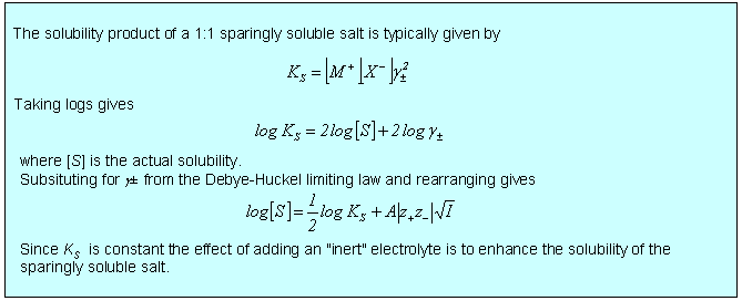
Electrolyte solutions present special difficulties because of the long range of the electrostatic interaction between ions. Coulomb's Law gives a force that varies as r−1 in comparison with van der Waals forces, which vary as r−6. The long range interaction means that an ion exerts an influence on ions that are a long way from it and hence on a large number of ions within a significant volume around it. This makes calculation of the effects of ionic charge on the free energy of mixing difficult. We start by considering the role of the dielectric constant in causing dissociation of a dissolved electrolyte. One can estimate that the dissociation constant of NaCl in the gas phase is 10−79. In water the Coulombic attraction of the two oppositely charged ions drops by a factor of 80 (the dielectric constant of water) and the dissociation constant changes to 7, i.e. NaCl dissociates fully in water. In a 0.1 M aqueous solution of NaCl the average distance between the fully dissociated ions is about 0.8 nm. However, in a solution of this concentration the Coulombic interaction between a pair of ions is similar to that between neighbours in comparable uncharged liquids at a distance of more like 3 nm. The Coulombic forces can therefore be expected to make strong contributions to both entropy and enthalpy of mixing.
The solution to this problem is known as the Debye-Huckel theory. This theory gives an expression for the activity coefficient as a function of electrolyte concentration, which is of considerable importance. You need to be able to use the Debye-Huckel result, known as the Debye-Huckel Limiting Law, and you should understand the qualitative issues behind it. The problem is as follows. A given central ion exerts a simple Coulombic force on ions in the first "shell of ions" but after this the Coulombic force is screened by this shell of ions and becomes progressively more screened as the distance increases. It would be possible to write an exact expression for the electric field for a given surrounding ion configuration. There are, however, two difficulties in doing this. First, the ions are undergoing thermal motion and so we must use an average smeared out distribution, and, secondly, the probability of finding ions at a given average distance from the central ion will depend on the Boltzmann factor. The Boltzmann factor depends on the energy of interaction and, since this depends on the electric field, we are back to where we started. Debye and Huckel broke the circle for dilute solutions. The first step in their results is that the potential around the central ion is a screened Coulombic potential with the simple form
ψ = (exp(−κr))/r
where κ is proportional to the square root of a quantity called the ionic strength (it is also inversely proportional to dielectric constant and temperature). The ionic strength isI = ½Σcizi2
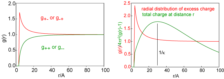
This equation for the potential leads to radial distribution functions for the two ions, which have the same shape as the potential and which are shown for a solution of 0.01 M 1:1 electrolyte on the left hand side of the figure below. In this figure the fact that the ions are hard spheres is also included, although this is not part of the original Debye-Huckel treatment. The fact that the hard sphere interaction is quite short compared with the range of the radial distributions illustrates the large range of the ion interactions in comparison with normal intermolecular forces. This can also be seen by comparing the radial distribution functions here with those given for neutral species earlier in the lecture course. The radial distribution for like charged ions shows a depletion that is exactly opposite to the extra ions present for unlike charged ions. Each of these contributes to the total charge surrounding an ion and the radial distribution for the nett charge is shown in the right hand side of the figure. The total charge about the central ion is obtained as a function of distance from the ion by integrating the excess nett charge, i.e. integrating (g(r) - 1)x4πr2 and the result of this is also shown in the right hand side of the figure. This distribution of charge shows that there is, on average, an atmosphere of charge surrounding a central ion. It is diffuse, it has a maximum at a distance of 1/κ, and the total charge integrated over r is equal and opposite to the charge on the central ion. This atmosphere of charge is called the ionic atmosphere and the distance 1/κ is often referred to as the radius of the ionic atnmosphere and/or the Debye length. Since κ is concentration dependent, through the equation given above, the Debye length is also concentration dependent. For a 1:1 electrolyte I = c and the Debye length varies as 1/c1/2. It is useful to remember that the Debye length is 10 nm for a 0.001 M solution of a 1:1 electrolyte. This collapses to 1 nm for a 0.1M solution, which is not very different from the average separation of ions estimated in the introductory paragraph. For a 1:2 or a 2:1 electrolyte it is easy to show that I = 3c and hence the radius of the ionic atmosphere drops by 1/31/2 on changing from a 1:1 to a 1:2 electrolyte of the same concentration.
The oppositely charge atmosphere interacts attractively with the central ion and hence lowers its free energy relative to an uncharged system. This lowering is greater the shorter the Debye length and the greater the charges of the ions involved. This leads to a lowering of the chemical potential and hence an activity coefficient less than one. Some care has to be taken in handling activity coefficients of electrolyte systems. Because charges can never be separated the activities (and activity coefficients) of electrolytes are given as geometric means, i.e. for a 1:1 electrolyte we use
μ = μ* + RTlnm± + RTlnγ±
where m±2 = m+m- and γ±2 = γ+γ-. Note that the standard state is the state with unit activity, not unit activity coefficient. The concentration is in mol dm-3. The Debye-Huckel limiting law is

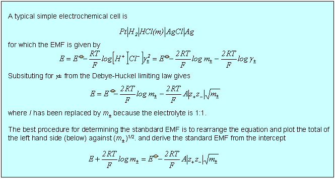
There is a wide variety of situations where the limiting law is very effective, three of which are considered below. In the first two cases, dissociation of a weak acid (or base) and solubility of a sparingly soluble salt, the qualitative effect is that the equilibrium is shifted because the ionic atmosphere stabilizes the ions and this stabilization is greater the greater the ionic strength. In the third case of the electrochemical cell, the limiting law provides a good quantitative means of accessing standard EMFs. There are several other situations involving electrochemical cells where the limiting law assists the quantitative determination of other thermodynamic parameters such as acid dissociation constants.
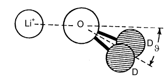
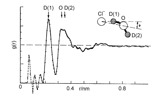
The Debye-Huckel theory does not take any account of ion hydration, although this starts to have a significant effect on activity coefficients at concentrations above about 0.2 M. There is a considerable body of evidence for the hydration of ions, much of it indirect. The most interesting and most direct comes from the determination of the radial distribution functions for elecetrolyte solutions which come from the use of neutron diffraction in conjunction with isotopic substitution methods. To describe the structure of water fully, requires the radial distribution functions, gHH, gOO, and gHO (= gOH). For an ionic solution even more are required. The way that these can be separately determined is by measuring diffraction patterns for different isotopic species, e.g.H2O and D2O. However, if only local structure is being examined some useful information may be obtained from more composite radial distribution functions. Two examples are shown below for the lithium and chloride ions. In each case, the radial distribution for H and O around the central ion is given for the ion in aqueous solution. The total hydration is obtained by integration, as described for simple liquids earlier in the course, and is 6 H2O for lithium and between 5 and 6 for chloride ion. From the positions of the peaks and the assumption that the geometry of the water molecule is unchanged from its free state the exact configuration of the hydrated waters can be determined. The angles marked in the diagram change with concentration.